Hello, world! My starting this blog has been long overdue. I thought I’d ease myself into it with something easy and uncontroversial, so here’s my take on linear regression. We start with the standard (frequentist) maximum likelihood approach, and show that Gaussian noise induces the familiar least-squares result, then show the correspondence between isotropic Gaussian priors and $l_2$ regularizers, before playing with some Bayesian updating using Mathematica. Note that these results are all well-known and discussed in detail in Bishop [1]; my motivation for reproducing them here is that I hadn’t encountered a concise and complete online write-up that I found satisfying.

Changelog:

2016-03-30: Edits for readability, and added a section on Bayesian regression.
2016-11-28: Some more minor edits, and moved the code to its own GitHub repo.

Setup

In the standard regression task we are given labelled data

\[\mathcal{D} \stackrel{\cdot}{=} \left\{\left(x_{i},y_{i}\right)\right\}_{i=1}^{N},\]

with each of the $y_i\in\mathbb{R}$, and $x_{i}\in\mathcal{X}$ drawn i.i.d. from some unknown stochastic process $\mu(x,y)$. Our objective is to learn a linear model $f:\mathcal{X}\to\mathbb{R}$ of the form

\[f(x;w,\phi)=w^T\phi(x),\]

where $w\in\mathbb{R}^D$ are our model weights (parameters), and the basis functions $\phi : \mathcal{X} \to \mathbb{R}^D$ are known and fixed. Now, let’s assume the data contains additive zero-mean Gaussian noise, so that

\[y(x)=f(x)+\epsilon \qquad \text{with }\epsilon\sim\mathcal{N}(0,\beta^{-1}),\]

and so the probability density of the targets conditioned on the inputs is

\[p(y|x,w) = \mathcal{N}\left(w^T\phi(x),\beta^{-1}\right).\]

The Gaussian noise assumption is motivated by the central limit theorem, and it helps in the Bayesian setting, since the Gaussian is its own conjugate prior. Note here that we make the conditional dependence on $x$ and $w$ explicit, and that we assume that the precision $\beta$ is known, and that the basis functions $\phi$ are well-chosen in some sense.

Maximum Likelihood Solution

Given that our dataset is drawn i.i.d., the likelihood is given by

\[\begin{aligned} p(\mathcal{D}|w) &= \prod_{i=1}^{N}p(y_i|x_i,w)p(x_i)\\ &= \prod_{i=1}^{N}p(y_i|x_i)\prod_{j=1}^{N}p(x_j)\\ & \propto \prod_{i=1}^{N}p(y_i|x_i)\\ &= \prod_{i=1}^{N}\mathcal{N}\left(w^T\phi(x_i),\beta^{-1}\right).\\ \end{aligned}\]

Our objective now is to learn the weights $w$ that maximise this likelihood, taking the variance of the noise $\beta^{-1}$ to be fixed. Notice that since the $p(x_{j})$ don’t depend on the parameters $w$, we can neglect them in our objective function. The maximum likelihood (ML) solution for $w$ is

\[\hat{w}_{\text{ML}} = \arg\max_{w}p(\mathcal{D}|w).\]

Now, $\log(\cdot)$ is a monotonically increasing concave function, so

\[\begin{aligned} \hat{w}_{\text{ML}}&=\arg\max_{w}\log p(\mathcal{D}|w)\\ &=\arg\max_{w}\log\prod_{i=1}^{N}\mathcal{N}\left(w^T\phi(x_i),\beta^{-1}\right)\\ &=\arg\max_{w}\sum_{i=1}^{N}\log\mathcal{N}\left(w^T\phi(x_i),\beta^{-1}\right)\\ &=\arg\max_{w}\sum_{i=1}^{N}\log\left(\frac{1}{\sqrt{2\pi\beta^{-1}}}\exp\left\{-\frac{\left(y_i-w^T\phi(x_i)\right)^2}{2\beta^{-1}}\right\}\right)\\ &=\arg\min_{w}\sum_{i=1}^{N}\left(y_i-w^T\phi(x_i)\right)^2.\qquad (1)\\ \end{aligned}\]

This shows the correspondence between maximizing the likelihood under Gaussian noise with minimizing the square error. Minimizing the sum of square error has a nice geometric interpration, since it corresponds to finding the point in the subspace spanned by the basis $\phi(x_i)$ which minimizes the Euclidean distance to $y_i$.

This is the standard frequentist result. The objective is a quadratic program, is convex, and has the well-known closed-form solution

\[\hat{w}_{\text{ML}}=\left(\Phi^T\Phi\right)^{-1}\Phi^Ty,\]

where $y$ is the vector of targets, and we have defined the design matrix $\Phi\in\mathbb{R}^{N\times D}$ so that its $i^{\text{th}}$ row is given by $\phi(x_i)$.

Maximum likelihood is notorious for overfitting, since by definition it finds the model for which our particular dataset is most probable; without tweaks, such a model will not generalize well to unseen data. The tweak that is typically introduced in the frequentist framework is an $l_2$ regularizer on the weights; this will tend to bias us towards simpler models with small coefficients. Note that there are numerous other ways in which we can penalize complex models; for example, we can use the MDL principle, or try to make $w$ sparse by using an $l_1$ regularizer instead.

MAP Inference

Interestingly, a certain class of prior over $w$ induces an $l_2$ regularizer when we calculate the posterior. This gives a stronger intuition for introducing this term into the objective function. Consider the isotropic Gaussian prior with hyperparameter $\alpha>0$

\[p(w|\alpha) = \mathcal{N}\left(0,\alpha^{-1}I_{N}\right),\]

where $I_N$ is the $N\times N$ identity matrix. Because a Gaussian is its own conjugate prior, we know that the posterior is a Gaussian. We can now easily compute the weights that maximize this posterior, conditioned on seeing some data $\mathcal{D}$. This is the maximum a posteriori (MAP) point estimate of $w$. Using the prior above, we can easily see that

\[\begin{aligned} \hat{w}_{\text{MAP}}&=\arg\max_{w}p(w|\mathcal{D})\\ &=\arg\max_{w}\frac{p(\mathcal{D}|w)p(w)}{p(\mathcal{D})}\\ &=\arg\max_{w}p(\mathcal{D}|w)p(w)\\ &=\arg\max_{w}\log\left(p(\mathcal{D}|w)p(w)\right)\\ &=\arg\max_{w}\left(\log p(\mathcal{D}|w) + \log p(w)\right)\\ &=\arg\min_{w}\left(\sum_{i=1}^{N}\left(y_i-w^T\phi(x_i)|\right)^2+\lambda\|w\|^2\right),\\ \end{aligned}\]

where the constant $\lambda(\alpha,\beta)$ is dependent only on the hyperparameters $\alpha$ and $\beta$. The second term in our objective is now clearly the $l_2$ regularizer we’ve been looking for. This objective is also convex, and has a simple closed-form solution analogous to the simple ML case.

Full Bayes

With MAP inference we start with a relatively ignorant prior over our model parameters, learn from a big batch of data, and end up with a point estimate. This clearly is not useful if we want to learn online with a sequential learning scheme, in which we update our belief $p(w)$ with each new datum we receive. For each new data point $d=(x,y)\in\mathcal{D}$ that we receive, we compute the posterior from Bayes rule, using as a prior the current state of our belief:

\[\begin{aligned} p(w|d)&=\frac{p(d|w)p(w)}{p(d)}\\ &=\frac{p(d|w)p(w)}{\int_{\mathcal{W}}p(d|w)p(w)\text{d}w}, \end{aligned}\]

where in our case $\mathcal{W}=\mathbb{R}^D$. Using Gaussian priors and likelihoods, we ensure that our posterior is also Gaussian, and so we can write down the posterior directly:

\[p(w|\mathcal{D})=\mathcal{N}(w|m_N,S_N)\]

where, as it turns out (Equations (3.53) and (3.54) in Bishop),

\[\begin{aligned} m_N &= \beta S_N \Phi^T y\\ S_N^{-1} &= \alpha I + \beta \Phi^T\Phi.\\ \end{aligned}\]

We now have the ingredients we need to implement a Bayesian updating scheme. The Mathematica notebook can be found here.

		$$\ \dots\ $$
(a)	(b)		(c)

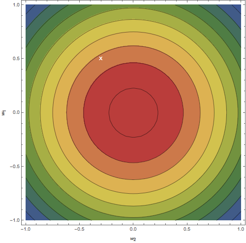
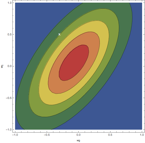
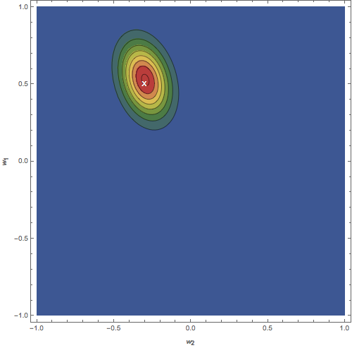
Figure: Contour plots of the distribution $p(w)$. (a) Isotropic prior. (b) Posterior after updating on one data point. (c) Posterior after updating on 20 data points. The white $X$ represents the ground truth.

Predictive distribution

We can use the predictive distribution, representing our uncertainty in the value of $y$, given some $x$ and a bunch of experience $\mathcal{D}$. Note that we marginalize out the parameter $w$, using $p(w)$.

\[p(y|x,\mathcal{D}) = \int_\mathcal{W}\text{d}wp(y|w,x,\mathcal{D})p(w)\]

Of course, the central issue with the Bayesian scheme (neglecting the computational/analytic difficulties arising from maintaining and updating a large distribution) is choosing the prior in a sensible and principled way. Note that the prior we used in the polynomial fitting example above was essentially chosen for convenience; though it is simple and thus reasonable according to Ockham’s principle, it is still chosen arbitrarily. Enter Solomonoff’s universal prior, which I’ll discuss more in a later post. $\square$

References

[1] C. M. Bishop. Pattern Recognition and Machine Learning. Springer, 2006