Bias-variance trade-off and the interpolating regime
A really nice paper went under my radar until my colleague Ian mentioned it recently in a tweet:
Looking back over the year, the one paper that gave me the best "aha" moment was...
— Ian Osband (@IanOsband) August 23, 2019
Reconciling Modern Machine Learning and the Bias-Variance Tradeoff:https://t.co/hubyXZATHQ
The "bias-variance" you knew was just the first piece of the story! pic.twitter.com/J24b0W8LDR
The motivation is the observation that in the modern ‘deep learning’ regime, we find empirically that large models generalize well even – especially – when trained to achieve zero loss on the training set. On the face of it, this seems to be at odds with the ‘sweet spot’ intuition that the bias-variance decomposition tells us. This paper uses some elegant experiments to connect these two observations – once the number of parameters exceeds some threshold (proportional to the size of the training set) we are in the ‘interpolating regime’, where the extra model capacity effectively allows us to interpolate between fitting data points smoothly; since smoothness is a property of many natural data distributions, this actually results in better generalization to the test set.
In this colab we’ll replicate the core experimental results from the paper. We’ll run two experiments: one to show the intuition with a toy example, and then one to reproduce the main result on MNIST.
![]()
Simple experiment
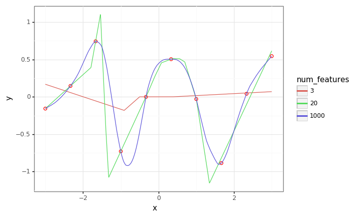
In this experiment, we flesh out the intuition in a simple setting, regressing linear models with random relu features. As we’ll see, as the we increase the number of features/parameters to greatly exceed the number of training points, we get a smooth interpolating fit, in contrast to what we see in the ‘classical’ regime, where \(\#\mathrm{parameters} < \#\mathrm{data}\).
# Always be importin'
from typing import Callable
import warnings

import numpy as np
import pandas as pd
import plotnine as gg
import sklearn

gg.theme_set(gg.theme_bw())
warnings.filterwarnings('ignore')
def random_relu_features(num_features: int) -> Callable[[np.ndarray], np.ndarray]:
  weights = np.random.randn(num_features, 2)

  def feature_fn(xs: np.ndarray) -> np.ndarray:
    n = len(xs)
    xs_with_bias = np.vstack([xs, np.ones(n)])
    return np.maximum(np.dot(weights, xs_with_bias), 0).T

  return feature_fn


def train_and_evaluate(
    train_xs: np.ndarray,
    train_ys: np.ndarray,
    test_xs: np.ndarray,
    feature_fn: Callable[[np.ndarray], np.ndarray],
    ) -> np.ndarray:

  train_features = feature_fn(train_xs)
  model = sklearn.linear_model.LinearRegression()
  model.fit(train_features, train_ys)

  test_features = feature_fn(test_xs)
  predictions = model.predict(test_features)

  return predictions
# Make some synthetic data.
num_data = 10
train_xs = np.linspace(-3, 3, num=num_data)
test_xs = np.linspace(-3, 3, num=1000)
train_ys = np.random.randn(num_data)
train_df = pd.DataFrame({'x': train_xs, 'y': train_ys})

# Train different models.
pred_df = pd.DataFrame()
for num_features in [3, 20, 1000]:
  feature_fn = random_relu_features(num_features)
  preds = train_and_evaluate(train_xs, train_ys, test_xs, feature_fn=feature_fn)
  df = pd.DataFrame({
        'x': test_xs,
        'y': preds,
        'num_features': num_features,
  })
  pred_df = pd.concat([pred_df, df])
plot = (gg.ggplot(train_df)
     + gg.aes(x='x', y='y')
     + gg.geom_point(size=2, color='red', fill='white')
     + gg.geom_line(data=pred_df, mapping=gg.aes(color='factor(num_features)'))
     + gg.labs(color='num_features')
)
plot
MNIST experiment
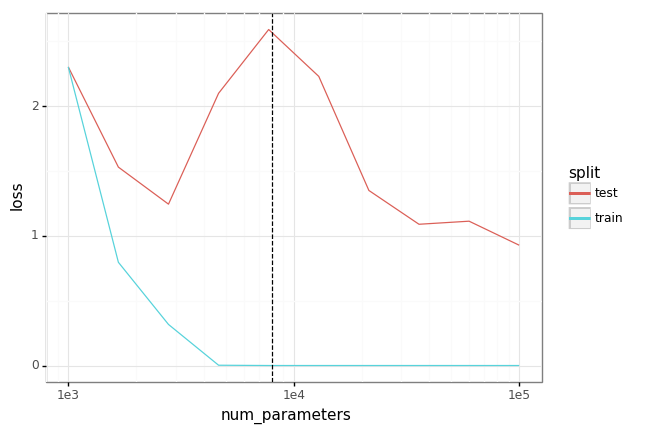
In this experiment we train a single hidden-layer MLP on MNIST for various sizes of the hidden layer. As the hidden size grows such that the number of parameters exceeds the number of training points (here a small subset of the whole MNIST training set), we see zero training loss + improving test set performance (the ‘interpolating’ regime). We also recover the classical ‘U’ risk curve in the ‘classical’ regime.
# We'll use TensorFlow 2 with Sonnet 2.
! pip install --quiet dm-sonnet
# @title Imports
import sonnet as snt
import tensorflow as tf
import tensorflow_datasets as tfds
# Hyperparameters and training setup.
num_data = int(4e3)
num_epochs = 1000
batch_size = 100
batch_size_eval = 1000
learning_rate = 1e-3
num_classes = 10  # MNIST.
input_dim = 784  # MNIST.
# Train & evaluation datasets.
data_train = tfds.load('mnist', split=tfds.Split.TRAIN, as_supervised=True)
data_train = data_train.take(num_data)
data_train = data_train.shuffle(num_data)
data_train = data_train.batch(batch_size)

data_eval = {
    'train': tfds.load('mnist', split=tfds.Split.TRAIN, as_supervised=True).batch(batch_size_eval),
    'test': tfds.load('mnist', split=tfds.Split.TEST, as_supervised=True).batch(batch_size_eval),
}
# Run the experiment.
results = []
for num_parameters in np.logspace(start=3, stop=5, num=10):

  # Create model.
  num_hidden = int((num_parameters - num_classes) / (1 + input_dim + num_classes))
  model = snt.Sequential([
      snt.Flatten(),
      snt.Linear(num_hidden),
      tf.nn.relu,
      snt.Linear(num_classes),
  ])

  # Create Adam optimizer.
  optimizer = snt.optimizers.Adam(learning_rate)

  # Initialize model weights.
  dummy_images, _ = iter(data_train).next()
  dummy_images = tf.image.convert_image_dtype(dummy_images, dtype=tf.float32)
  model(dummy_images)

  @tf.function
  def train(images: tf.Tensor,
            labels: tf.Tensor) -> tf.Tensor:
    images = tf.image.convert_image_dtype(images, dtype=tf.float32)
    with tf.GradientTape() as tape:
      logits = model(images)
      loss = tf.nn.sparse_softmax_cross_entropy_with_logits(logits=logits, labels=labels)
      gradients = tape.gradient(loss, model.trainable_variables)
      optimizer.apply(gradients, model.trainable_variables)
    return tf.reduce_mean(loss)

  @tf.function
  def evaluate(images: tf.Tensor, labels: tf.Tensor) -> tf.Tensor:
    images = tf.image.convert_image_dtype(images, dtype=tf.float32)
    logits = model(images)
    loss = tf.nn.sparse_softmax_cross_entropy_with_logits(logits=logits, labels=labels)
    return tf.reduce_mean(loss)

  # Training.
  for epoch in range(num_epochs):
    for images, labels in data_train:
      train(images, labels)

  # Evaluation.
  for split, dataset in data_eval.items():
    images, labels = iter(dataset).next()
    loss = evaluate(images, labels)

    result = {
        'num_parameters': num_parameters,
        'split': split,
        'epoch': epoch,
        'loss': loss.numpy(),
    }
    print(result)
    results.append(result)

df = pd.DataFrame(results)
plot = (gg.ggplot(df)
     + gg.aes(x='num_parameters', y='loss', color='split')
     + gg.geom_line()
     + gg.scale_x_log10()
     + gg.geom_vline(gg.aes(xintercept=num_data*2), linetype='dashed')
)

plot
Post script: literally as I was finishing this post, Pedro Domingos tweeted on the same topic!
Old: Memorizing the data is overfitting.
— Pedro Domingos (@pmddomingos) October 11, 2019
New: Memorizing the data is essential for good generalization.